Requisite Simplicity
Contemporary complexity science theoryComplex System and Complexity Science
Systems can be categorized as either simple, complicated, or complex. While simple and complicated systems can be intricate, their behavior can be ascertained from the properties of their constituent parts. Such an assessment is not possible for complex systems which exhibit ‘system complexity.’ After Cilliers (1998) and Cilliers et al. (2013), we define system complexity by particular characteristics of a system that arise because of interconnections, interactions, and nonlinear relationships among system elements. System complexity is an emergent property of the entire system rather than the individual elements. These peculiar properties emerge at the system level because complex systems cross multiple domains (i.e., natural, societal, political) and scales (i.e., space, time, jurisdictional, institutional) (Islam and Repella 2015). Therefore, it is nearly impossible to predict the behavior of a complex system by reducing it to its constituent parts and studying them in isolation. This inadequacy of reductionist approaches to describe system behavior is at the heart of our distinction between complex systems and those that are merely simple or complicated. Figure 1 presents a comparison between aspects of simple, complicated and complex systems adapted from the Cynefin framework proposed by Snowden and Boone (2007).
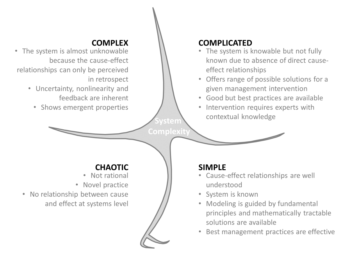
Figure 1: Cynefin framework showing distinction between simple, complicated and complex system (Adapted from Snowden and Boone 2007; Islam and Repella 2015)
To cite the text above and know more about the complexity science and concept of requisite simplicity, please visit:
Palash, W., K.M. Smith, and S. Islam, 2019: Coupling of Natural and Human Systems: A Case Study of a Complex System from Southwest Bangladesh Delta. Interdisciplinary Collaboration for Water Diplomacy: A Principled and Pragmatic Approach, S. Islam & K. Smith Eds., Routledge (Taylor & Francis), New York, USA.
Requisite Simplicity
Two different considerations must be considered to understand the limits of flood forecasting accuracy: a catchment condition that focuses on the state of the catchment and an atmospheric condition that examines the predictability of precipitation inputs. Not surprisingly, precipitation, a key input to a flood forecasting model, is generally considered to be the largest source of uncertainty for medium- to long-range flood forecasting (Pappenberger et al. 2005; Bauer et al. 2015; Wu et al. 2017). Accuracy of flood forecasting models, whether using observed or forecasted rainfall, are also limited in their ability to capture local characteristics of the rainfall–runoff processes because we do not know the soil and geological properties of catchments at the scale needed to model the relevant dynamics (Marks and Bates 2000; Pappenberger et al. 2005). In fact, the recognition of fundamental problems in the application of physically based models—due to scale mismatch between model equations and heterogeneity of rainfall and runoff-generating mechanisms; practical constraints on solution methodologies; and uncertainties associated with parameter estimation, model calibration and validation— for flood forecasting is not new (Beven 1989; Wood et al. 2011; Beven 2012).
A flood forecasting system usually includes a large number of nonlinear relationships among rainfall and runoff processes with feedback. To generate a perfect (or nearly perfect) model of such a system, one has to model everything (or nearly everything). Yet, as Lorenz (1963) aptly pointed out, in a nonlinear system with feedback, approximate accurate representation of the present does not guarantee accurate forecast of the future due to sensitivity to the initial conditions. Consequently, to develop a reliable and robust flood forecasting model, we have to reduce the complexity of processes, interactions, and feedback by simplifying the model structure. Currently, we do not have a generally accepted criterion to decide what constitutes a simple model within the context of complexity of modeling and functional utility
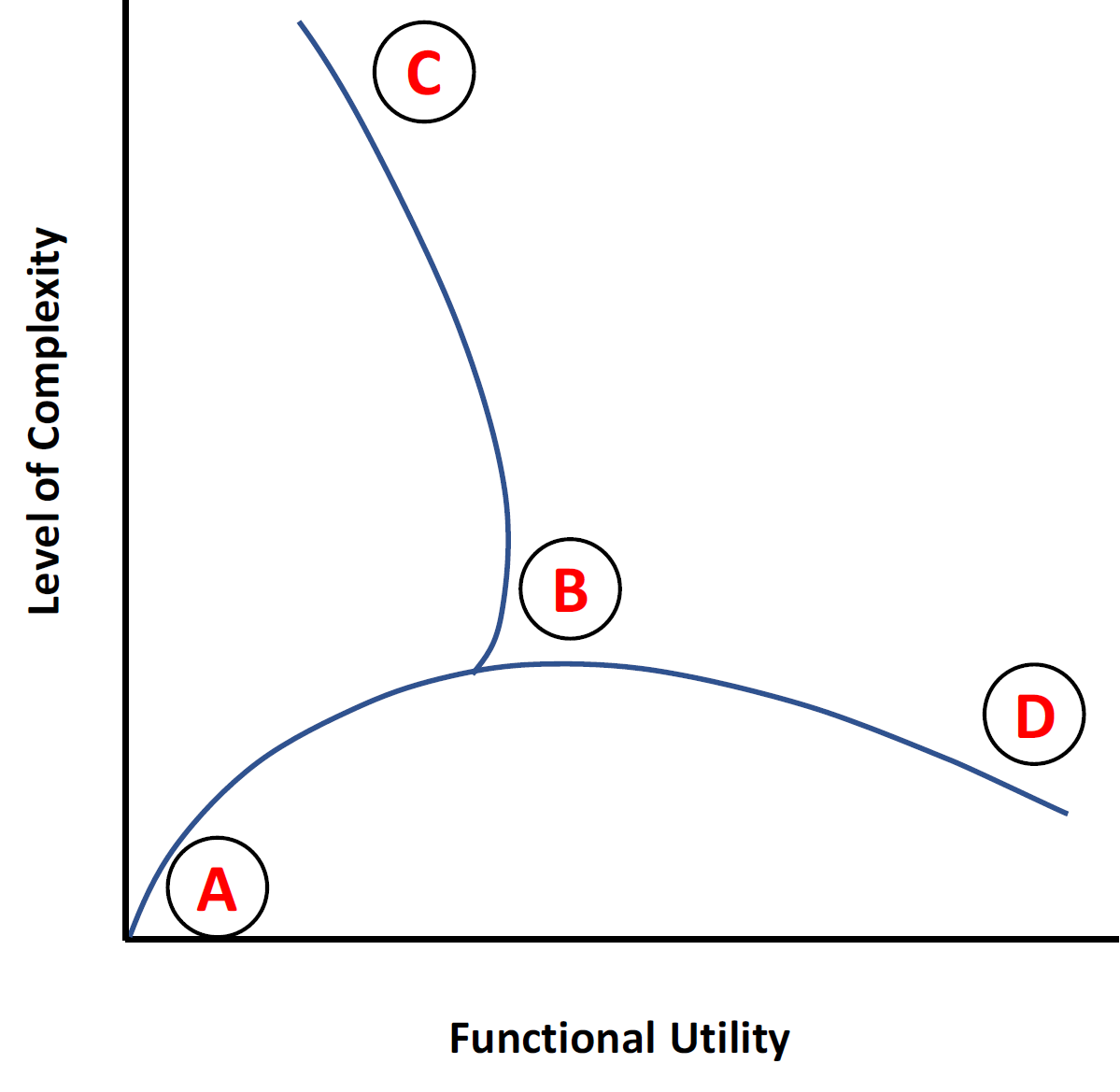
Figure 2: Requisite simplicity trade-off between modeling complexity and functional utility (adapted from Ward 2005).
We adapt an approach proposed by Ward (2005), in the context of system design, to illustrate the relationship between modeling complexity and functional utility (Figure 1.2). We begin at the lower left quadrant in region A. Here the system is simple: cause–effect relationships are known, modeling is guided by fundamental principles, and mathematically tractable solutions are usually found. As we introduce more realism to our model, we move toward region B. During this move, new variables, processes, and dynamics are introduced. An increased level of modeling complexity—from region A to B—thus usually leads to better functional utility (e.g., forecasting accuracy). At this stage, we may have a functional flood forecasting model for a given purpose. Further increasing the level of model complexity, however, may not lead to better forecasting accuracy.
Over the last several decades, with an advanced understanding of atmospheric physics, deployment of a global upper-atmospheric observation network, and increased computational power, our ability to provide skilled short-term (1–5 days) precipitation forecasts has improved. However, Lorenz (1963)—in his pioneering work on chaos—showed that nonlinear systems are only predictable for a finite time owing to their sensitive dependence on initial conditions. This puts a fundamental limit on our ability to provide accurate medium-range (5–10 days) precipitation forecasts. For example, a careful examination of over 40 years of 8-day atmospheric forecasts over the contiguous United States (e.g., Clark and Hay 2004; Cloke and Pappenberger 2009) or the European Centre for Medium-Range Weather Forecasts (ECMWF)-generated precipitation forecasts over the Danube basin (Pappenberger and Buizza 2009) suggests a limit on the predictability of precipitation with very low to modest skill out to 4–5 days. Given that the antecedent conditions likely dominate the runoff over lead times shorter than the time to concentration of the basin (Voisin et al. 2011), moderately skillful numerical precipitation forecasts at such short lead times may not lead to better forecasting accuracy. However, there is a perception that increased forecasting accuracy is achievable by simply increasing the space–time resolution and physical parameterization of numerical models. This perception may lead one to a journey from region B to C, in which model complexity increases without any appreciable change in functional utility.
While in region B, further progress may come not from adding more modeling complexity, but from simplification. Here, we argue that simplification may be achieved as we move from region B to D by taking a closer look at the dominant processes for large river basins and reducing the model to its essential components. The proposed requisite simplicity—to paraphrase Einstein, ‘‘simple but not simpler’’—is achieved by identifying the key components of the rainfall–runoff process and developing ways to track their evolution for our ReqSim flood forecasting models described in ReqSim Model page of this current site.
To cite the text above and know more about the concept of requisite simplicity, please visit:
, 2018: A Streamflow and Water Level Forecasting Model for the Ganges, Brahmaputra, and Meghna Rivers with Requisite Simplicity. J. Hydrometeor., 19, 201–225, https://doi.org/10.1175/JHM-D-16-0202.1
Application
Will be updated shortly.