ReqSim Model

To cite the text below and know more about the ReqSim modeling framework, please visit:

Palash, W., Y. Jiang, A.S. Akanda, D.L. Small, A. Nozari, and S. Islam, 2018: A Streamflow and Water Level Forecasting Model for the Ganges, Brahmaputra, and Meghna Rivers with Requisite Simplicity. J. Hydrometeor., 19, 201–225, https://doi.org/10.1175/JHM-D-16-0202.1

Approach  

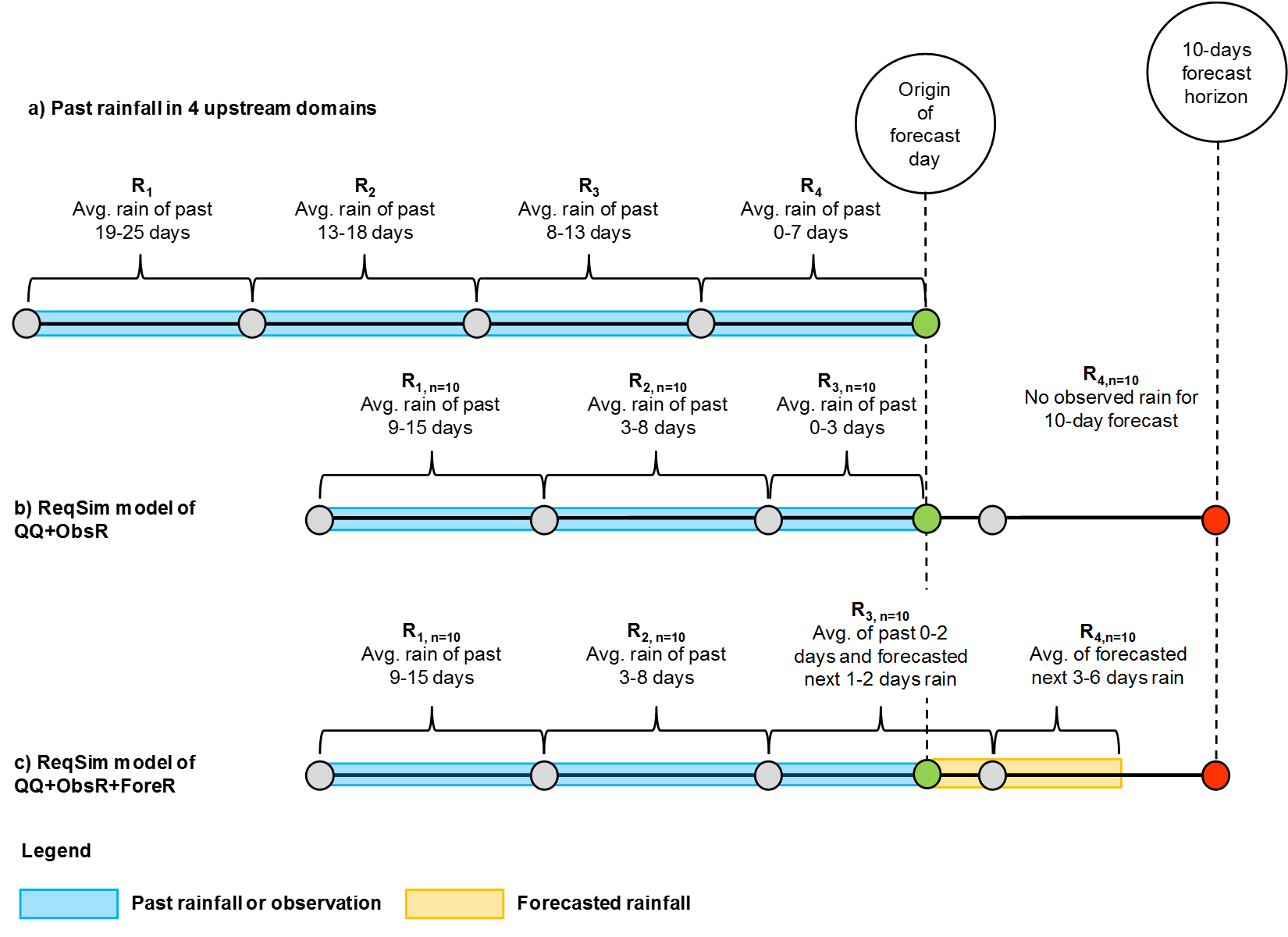
Illustration of the ReqSim model structure of the Ganges basin. Upstream rainfall aggregation for (a) today’s Ganges flow, (b) for 10-day Ganges forecasts using the QQ+ObsR model, and (c) 10-day Ganges forecasts using the QQ+ObsR+ForeR model.

where,  X_t and X_t+k are streamflow data at time t and t+k separated by lag k;  μ and σ are mean and standard deviation of streamflow X. We considered the river flow as second order stationary with constant mean and variance.

The strong persistence of daily streamflow up to several days provides the opportunity of using persistence based QQ model. A simple QQ model, therefore, is:

where, Q_t+n is the forecasted streamflow or WL of n-day lead time; Q_t and Q_t-1 are observed streamflow or WL on forecast day t and previous day t-1, respectively; α_n and β_n are model coefficients related to persistence; and γ_n is regression interception coefficient.

Flow Persistence + Obs Rain

A detailed mechanistic rainfall-runoff transformation model is desirable to convert upstream rainfall to downstream flow conditions. Given the size of the basin, lack of detailed data from upstream regions and difficult of calibrating and validating model parameters for such a model, we opted to use a simple linear transformation of rainfall to runoff. Division of entire basin into four large domains and their corresponding flow travel time to downstream forecast locations (see Section 2.2 in Palash et al. 2018) help us to calculate daily space aggregated (i.e., averaging domain-wide rainfall) and then time aggregated (i.e., averaging daily domain rainfall from minimum to maximum flow travel time) rainfall by using Eq. (4). For example, our isochrones analysis shows that runoff from most upstream domain of the Ganges (domain I) located in the western Ganges takes up to 19-25 days to arrive at Hardinge Bridge (HB) in Bangladesh (Figure 1). In other words, rainfall that occurs in the Ganges domain I 19-25 days before has a contribution to current Ganges flow at HB. Similarly, runoff from domain II of the Ganges may take 13-18 days, from domain III 8-12 days and from domain IV 0-7 days to arrive at HB. Therefore, we averaged domain I, II, III and IV’s past daily rainfall of 19-25 days, 13-18 days, 8-12 days, and 0-7 days to get the space-time aggregated rain signal , ,  and , respectively which can be considered linearly correlated to current HB flow. A similar approach has been applied to the Brahmaputra and UM (Barak) basin for calculating their space-time aggregated domain rainfall.

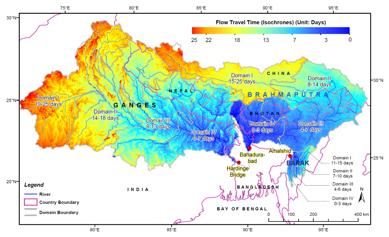
Figure 1: Isochrones of the GBM basin with flow travel times of the four large domains.

It is important to note that when space aggregated daily rainfall is compared against downstream daily streamflow of the basin, it is hard to establish any direct ‘linear’ relationship between the two due to noise in daily rainfall (left panel of Figure 2). But, if we compare space-time aggregated domain rainfall with applying average flow travel time lag of each domain then the rainfall becomes more correlated to downstream streamflow (right panel of Figure 2). Hence, a space-time aggregating process helps to establish a ‘near’ linear correlation between upstream domain rain and downstream streamflow (i.e., high upstream rain to high downstream streamflow or vice versa). The regression structure of the ReqSim model utilizes the same ‘linear’ correlation in its parameter estimation and prediction. The ReqSim model structure Figure (a) (at the top of this page)  shows how downstream flow of the Ganges on the day of forecast responds to past rain signals of four upstream domains, while Figure (b) illustrates the predicted response of downstream flow at 10-day forecast horizon given observed rainfall within three upstream domains. The fourth or most downstream domain does not contribute to the 10-day forecast because its time of concentration is shorter than the forecast window.

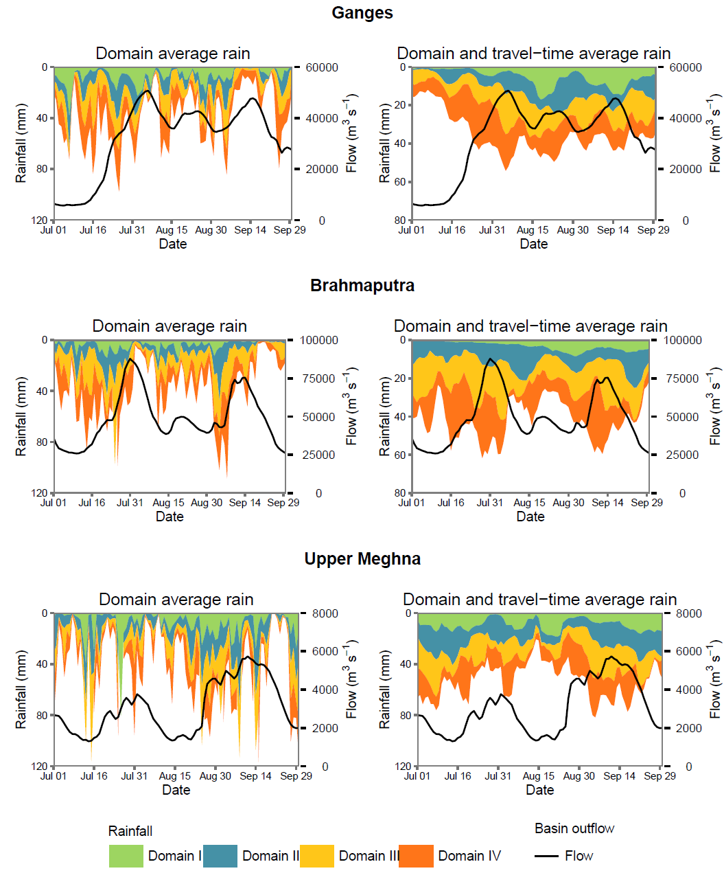
Figure 2: GBM flow with domain-average upstream rainfall during the 2007 monsoon. The domain rainfall is plotted on the primary y axis with values in reverse order, while the downstream daily flow at forecast locations is on secondary y axis. (left) Daily domain-averaged (space aggregated) rainfall compared with downstream daily streamflow at the forecast location. (right) Domain and flow travel time-averaged (space–time aggregated) rainfall compared with downstream daily streamflow at the forecast location.

Because of a relatively large lag time between the upstream rainfall and corresponding downstream streamflow in a large river basin like the Ganges, upstream rainfall has the potential to be a good predictor of downstream flow (Akhtar et al., 2009). This observation provides the rationale of incorporating upstream observed rain (ObsR) information into the flow persistence or QQ model to develop the flow persistence with observed rainfall (QQ+ObsR) model. The structure of the QQ+ObsR model is: 

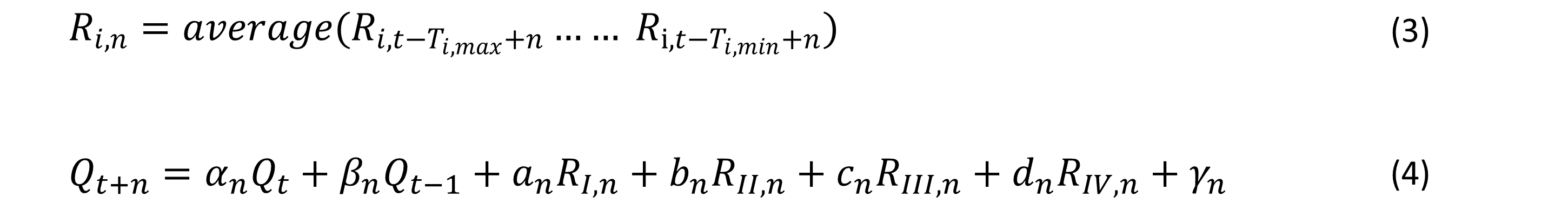
Where Q_t+n, Q_t, Q_t-1, α_n, β_n, γ_n, and n denote the same as Eq. (1); R_I, R_II, R_III and R_IV are lagged space-time aggregated domain rainfall of domain I, II, III and IV, respectively (Figure 1 and 2); and a_n, b_n, c_n, d_n are model coefficients related to upstream rainfall of each of four domains. T_i,max and T_i,min are maximum and minimum flow travel time (in days) for domain I (I to IV) while t is the forecast day (i.e., 0 day), and n is the forecast lead time (1 to 10-day). If t-T_i,max+n and/or t-T_i,min+n > t then observed rainfall data up to forecast day is considered in the QQ+ObsR model. For example, let’s assume we want to generate Ganges forecasts for 10-day lead time; so, n = 10 and forecast day t = 0. Calculating rainfall for domain III of the basin (flow travel time is 8-13 days) would require rainfall from (0 – 13 + 10) days to (0 – 8 + 10) days rain, i.e. 3 days past rainfall to 2 days future rainfall. Since, QQ+ObsR model does not consider forecasted rain to its regression, domain III rainfall calculation includes rain from past 3 days only, i.e., no future rain is considered.

Flow Persistence + OBS Rain + Fore Rain

The structure of QQ+ObsR+ForeR model is similar to the QQ+ObsR model; the only difference is it uses the forecasted rain (ForeR) into its regression equation along with the ObsR. For example, if t-T_i,max+n and/or t-T_i,min+n > t where t is the forecast day (i.e., 0 day) then forecasted rain of m lead time is considered in QQ+ObsR+ForeR model for domain i providing that t-T_i,max+n and/or t-T_i,min+n ≤ t+m. The ReqSim model structure figure (at the top of this page) demonstrates the 10-day (i.e., n = 10) Ganges forecasting process by using 6-days forecasted rain (i.e., m = 6) applied in QQ+ObsR+ForeR model.

Data

We used historical records of daily measured WL and rated discharge data of 30 river points in Bangladesh including HB (Ganges), Bahadurabad (Brahmaputra), and Amalshid (UM– Barak) in our model. We collected these data from Flood Forecasting and Warning Center (FFWC) of Bangladesh Water Development Board (BWDB) and Institute of Water Modelling (IWM) over 1998–2019. FFWC calculates rated discharge by applying measured WL-discharge rating equations (Hopson and Webster 2010). We also considered three sets of gridded rainfall data: first, the near real-time observed rainfall data of Tropical Rainfall Measuring Mission (TRMM) 3B42V7 with 0.25⁰ resolution over 1998–2019, second, 1–6-day forecasted rainfall for 2014–19 generated by the Weather Research and Forecasting (WRF) Model and collected from IWM, Bangladesh, and third, the Global Forecast System (GFS) generated forecasted daily rainfall data up to 10-day lead-time (spatial resolution 0.25⁰) collected from Research Data Archive (RDA) for 2015-19.